Bayesian Networks

I have mentioned before that Bayesian Inference is, in general, intractable. People like Gaussians a lot because many nice results in closed-form can be derived from them, analytical treatments are in general possible and even easy to do, but for more general distributions you need a lot of information in order to perform useful inference.

Consider, for instance, the triparametrised Student’s t-distribution which I talked about in two posts of mine. Unlike the normal distribution, which has very neat closed forms for calculating many aspects of it, we can’t find a closed-form solution for its Maximum Likelihood Estimation or its Maximum A Posteriori value. There are iterative algorithms to calculate these things, sure, but they have to be applied case-by-case.

Even that is not what I mean by “intractable,” though. I think the best example we can use is that of a few discrete binary variables. We know from Bayes’ Theorem that, for any two variables and , , whence to infer the value of after having observed we need to calculate .

Now suppose we’re dealing with four binary variables, , , , and , and we have a joint distribution table for them (that is, a table with the values of and and and so on for every possible combination). Then, in order to calculate and perform inference, we need:

(That is the tiniest size can render anything on my blog, and it still wasn’t enough.)

To make the above clearer, I’ll rewrite it:

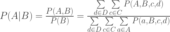
Where I’m shorthanding for . We have to sum over all possible values of the other variables.

The numerator, then, is a sum of terms. The denominator is a sum of terms. This suggests a general rule, which is correct: if we’re dealing with binary variables, then simple inference of the value of one of them when the value of another has been observed requires terms to calculate the numerator and terms to calculate the denominator. For small values of , this is not too bad, but this calculation takes exponentially many steps to be performed.

Not to mention the exponentially many memory entries necessary to even have the table! As you might’ve noticed, we need to store values (the there is because they all must necessarily sum to , so the last value can be deduced from the other ones) in the table. And usually, we’re dealing with much more than variables, and stuff gets complicated really fast when numbers start growing.

(No, really fast. Like, I’m fairly good at maths and the table of the time it takes to do breadth-first search in a tree as a function of its depth is still breathtaking:

Consider that we can have wayyyyy more than variables in an inference problem and you can surely understand why this can be fairly hard.

(Well this is not a completely fair comparison, breadth-first search takes much more time than Bayesian Inference in binary variables, but my point was just how fast exponential complexity is, really, in practical terms.))

And even this analysis is not complete, since full Bayesian treatment of real life would involve a Solomonoff prior over every possible reality, and that is literally uncomputable, amongst other complications even when we ignore the above. Just trying to give you a taste of what I mean.

We need some way of making this easier on us. One such way is a Bayesian Network.

---

Informally, a Bayesian Network is a graphical model that represents dependencies and lack thereof in a set of variables. I’ll explain this with an example, the universal example to explain Bayes Nets:

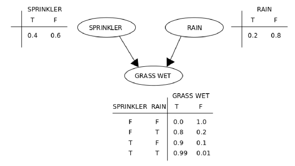
Suppose that there are two events which could cause grass to be wet: either the sprinkler is on or it’s raining. Also, suppose that the rain has a direct effect on the use of the sprinkler (namely that when it rains, the sprinkler is usually not turned on).

A Bayes Net treats the above problem with two tools: a graphical model and a few conditional probability tables. For the above example, one possible representation is given by:

So , , , and so on. Note that, since the first and second columns of each table above must sum to on each line, the table really only has values. That’s exactly as many values as a full joint distribution would have, but this is because this graph is fully connected: every node is connected to every other node.

Suppose the sprinkler’s rain detection system is busted, and it can no longer tell when it’s raining. The above would then change to:

Note that now the full conditional table has one less entry, since the sprinkler’s activation no longer depends on the rain. So the biggest advantage, here, is exactly in the independencies encoded in a Bayes Net. The change becomes more pronounced the more variables we have, but in general inference is easier with a Bayes Net.

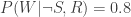
Suppose, for instance, that I know the grass is wet, and I want to know whether it’s raining and the sprinkler is off. In a fully general sense, with the joint probability table, I’d have to calculate:

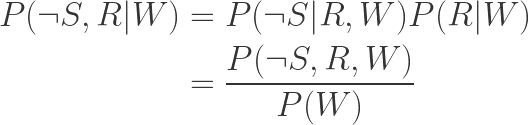
And that last term would have that annoying sum over all possible values of sprinkler and rain in the denominator. However, with the Bayes Net, I have the conditional probability tables, and I have the independency , whence:

All the values in the numerator are stored directly in the tables, and the denominator can be calculated from the tables of the three variables.

Now, this may seem like not that much of a gain, since the denominator still has exponentially many terms that we need to sum over. However, Bayesian Networks have another property that’s not shown in that table which is the Local Markov Property. Basically, they’re “local,” in the sense that to calculate the probabilities of a node, you only need its values and the values of things directly linked to it.

For example, suppose my Bayes Net is actually like this:

(Before anything, note that this table has entries, where a fully general joint distribution over four binary variables would have entries.)

In this case, the sprinkler doesn’t detect the rain, but rather whether it’s cloudy. Or maybe it doesn’t detect that either, maybe there’s a gardener who sees that it’s cloudy and turns off the sprinkler when that happens. Anyway, what I want you to see is that the grass probability table is still the same size. The new variable, “cloudy,” affects it not at all, because sprinkler and rain are in the way.

So while before we’d have to sum over all possible values of the grass for all possible values of sprinkler, rain, and cloudy in the denominator, with this Bayes Net we can safely ignore cloudy. Yes Bayesian Inference is still exponential in the variables involved, but the independencies encoded in the Bayes Net ensure that “the variables involved” are only those directly linked to whatever we’re interested in. Stuff is strictly local, and there is significant gain in computation.

Of course, there’s still the problem that, even if local, inference is still exponentially complex, and the power of the Bayes Net depends very strongly on how many independencies are encoded by it. But still, it helps quite a bit.

---

More formally, let be a set of random variables in the Bayesian sense, and a joint probability density (or mass) function over . Let be a directed acyclic graph, where is the set of vertices of the graph (with the property ) and is the set of directed edges of the graph (with the property that the graph contains no cycles). For every , let be the set of all vertices whose outgoing edges point to (we call that set the set of parents of ). Then is a Bayesian Network with respect to if  can be written as

where is the unique variable associated with and is the set of variables associated with the parents of . We will refer to and as the same thing, for ease of notation.

The above definition entails both discrete, continuous, and hybrid Bayesian Networks, and entails the Local Markov Property as well, which states that every variable in a Bayesian Network is independent of its non-descendants conditional on its parents.

Bayesian Networks are sometimes used in Machine Learning for classification problems, and sometimes even for regression problems. However, very few people actually work with them as, even though they are a significant improvement over fully general Bayesian Inference, exact inference in Bayes Nets is still not very tractable (in fact, it is NP-hard), and even approximate inference is intractable.

Its greatest advantages, in addition to the technical ones, are ease of use and intuitiveness – their meaning tends to be clear at a glance. This in fact is how I mostly use them, as intuition pumps and demonstration tools. However, I will write further in the future about inference in Bayes Nets and its applications for Machine Learning.